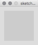
Output from the Processing Development Environment are put to the Display Window (DW).
The DW is measured in Pixels in a grid of tiny square dots, the smallest element that can be represented on a computer's display screen.
The grid of pixels is measured from the upper left corner starting with 0,0 to the lower right corner with width-1, height-1. That's because its easier to do math in computer coding when you start counting from 0 instead of 1. (There's even a technical name for math errors in code because of this oddity: "OFF By One Error")
PROCESSING
Extra 3-1: Draw a Window (1)
size(100, 100);
PROCESSING
Extra 3-1: Draw a Window (2)
size(500, 500);
PROCESSING
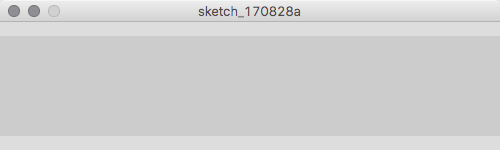
Extra 3-1: Draw a Window (3)
size(500, 100);
Draw A Point
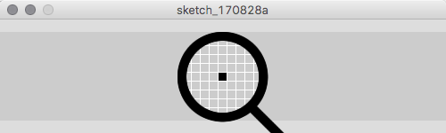
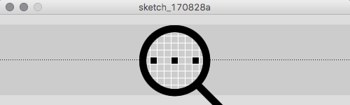
We can set any pixel in the DW with point(x,y), where x and y are the coordinates of the point
PROCESSING
Extra 3-2: Draw a Point
size(500, 100);
point(250,50);
PROCESSING
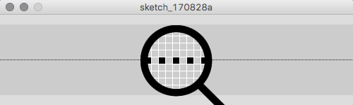
Extra 3-2: Draw a Point Animated
int x = 0;

void setup() {
  size(500, 100);
}

void draw() {
  point(x, 50);
  x = x + 2;
}
PROCESSING
Extra 3-2: Draw a Point Animated with More Space
int x = 0;

void setup() {
  size(500, 100);
}

void draw() {
  point(x, 50);
  x = x + 3;
}
Basic Shapes
PROCESSING
Example 3-3: Draw a Line
size(200, 200);
line(10, 10, 90, 90);
line(x1, y1, x2, y2)
starting location x, starting location y,
ending location x, ending location y
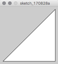
triangle(x1, y1, x2, y2, x3, x4)
point 1 location x, point 1 location y,
point 2 location x, point 2 location y,
point 3 location x, point 3 location y
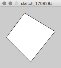
quad(x1, y1, x2, y2, x3, y3, x4, y4)
point 1 location x, point 1 location y,
point 2 location x, point 2 location y,
point 3 location x, point 3 location y,
point 4 location x, point 4 location y,
PROCESSING
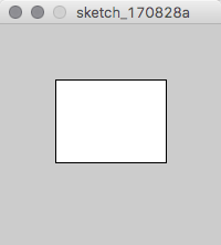
Basic Shapes: Rect
size(200, 200);
rect(50, 50, 100, 75);
rect(x, y, w, h)
origin location x, origin location y,
width, height
PROCESSING
Basic Shapes: Ellipse
size(200, 200);
ellipse(100, 100, 150, 150);
ellipse(x, y, w, h)
origin location x, origin location y,
width, height
This is a weird one. It measures out in units of Pi, called radians, and the starting point on the ellipse is on the far left edge. arc(x, y, w, h, start, stop)
origin location x, origin location y,
width, height
start, stop - in radians!
Here's a version of arc() using the function radians(N) that will return a value of PI for a given value of N degrees.
There's something peculiar about this too. Can you tell what it is?
Drawing Order
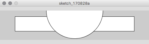
It matters what sequence you write out the code as to how a shape will be displayed relative to another shape. The later in the sequence in the code, the higher in the layering order, or the more on top it will be
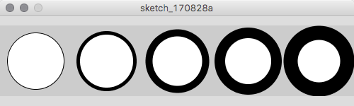
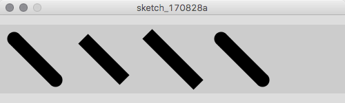
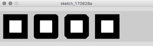
The default is MITER. The values for strokeJoin() must be (in capital letters only): ROUND, BEVEL, MITER.
Drawing Modes
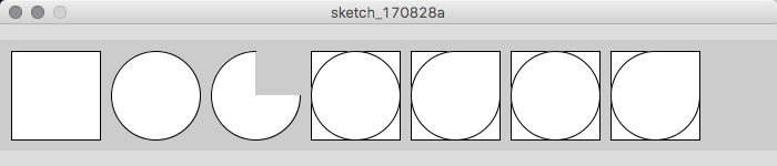
Another oddball gizmo for ellipses and arcs. By default, ellipses and arc are positioned by their centers. But you can change them to be drawn from their upper-left corner with ellipseMode(CORNER). The default mode is ellipseMode(CENTER), and there's even a way to do it by both corners (ellipseMode(CORNERS), which sets the upper left and lower right x,y values, rather than the width and height.
There's several ways of declaring a color, and functions that will take a color value:
background()
fill()
stroke()
color() - this is a special way of storing a color in a variable, more later...
Colors can be identified in one of two ways: as a gray value from 0 to 255 (28), or as an color value with varying shades of each color value for Red, Green, and Blue (RGB), also measured in values from 0 to 255. (NOTE: There's other ways to control color with colorMode(), but never mind for now. The good news is, if you're used to hexadecimal colors for the web, you can use those too.)
PROCESSING
Spec Color: Black
size(200,100);
background(0);
PROCESSING
Spec Color: Gray
size(200,100);
background(128);
PROCESSING
Spec Color: White
size(200,100);
background(255);
PROCESSING
Spec Color: Red
size(200,100);
background(255, 0, 0);
PROCESSING
Spec Color: Purple
size(200,100);
background(128, 0, 128);
PROCESSING
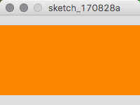
Spec Color: Orange
size(200,100);
background(#FF8800);
Hexadecimal Color
Hex color is fairly easy once you get used to it, probably a bit easier to work with, and easy to look up on the web and easier to cut and paste.
Hexadecimal numbers are annoted with the digits 0 thru 9, but since it's actually base 16 instead of 10, it uses A, B, C, D, E, and F to represent the numbers 10 thru 15.
Decimal
Hexadecimal
Decimal
Hexadecimal
Decimal
Hexadecimal
0
0
9
9
32
20
1
1
10
A
33
21
2
2
11
B
72
48
3
3
12
C
108
6C
4
4
13
D
128
80
5
5
14
E
255
FF
6
6
15
F
7
7
16
10
8
8
17
11
In Hex color, there's three sets of hexadecimal values consisting of two characters each. So when we see:
#FFFFFF
We see white because the first set 'FF' tells the Red value of RGB to be full on, the second 'FF' tells Green to be full on, and the third 'FF' tells Blue to be full on
Hex
RGB
Result
Red
Green
Blue
#FFFFFF
FF
255/255, 100%
FF
255/255, 100%
FF
255/255, 100%
White
#FF0000
FF
255/255, 100%
00
0/255, 0%
00
0/255, 0%
Red
#00FF00
00
0/255, 0%
FF
255/255, 100%
00
0/255, 0%
Green
#0000FF
00
0/255, 0%
00
0/255, 0%
FF
255/255, 100%
Blue
#FFFF00
FF
255/255, 100%
FF
255/255, 100%
00
0/255, 0%
Yellow
#FF8000
FF
255/255, 100%
80
128/255, 50%
00
0/255, 0%
Orange
#EEE5D3
EE
238/255, 93.3%
E5
229/255, 89.8%
D3
211/255, 82.7%
Tan-ish
Fills & Strokes
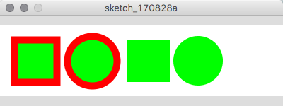
fill() and stroke() define the obvious fill and stroke of a shape. You can also turn oFF a stroke entirely with noStroke().
If trying to figure out that dark orange is fill(128, 0, 0) is not something that you can easily remember, or that puce is fill(114, 47, 55), then be glad that Processing has a built-in color picker.
Setting Transparency
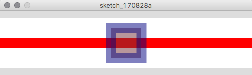
By adding a fourth parameter to a defined RGB color (or a second one to a grayscale color) you can control the transparency of a shape
There's more shapes that can't be drawn with point(), line(), rect(), quad(), ellipse(), and arc() than can be.
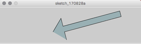
One way to draw a more complex shape (but one without any curves) is to use vertex() combined with beginShape() and endShape(). A vertex() is defined by an x and y coordinate in the Display Window
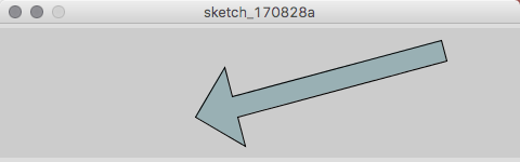
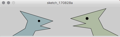
The best way to plot these out in on graph paper with a pencil. In our book they have an example, let's try it...
And, Processing has one more trick up its sleeve. If you don't create a shape with beginShape() and endShape() that is closed (that is, the last vertex isn't the same as the first vertex), then you can add a property to endShape(CLOSE) to close the shape.
Do you see the pattern of something(ALLCAPS)? The text in ALLCAPS is a called reserved word, or a property that's pre-defined by the Processing language. Things like:
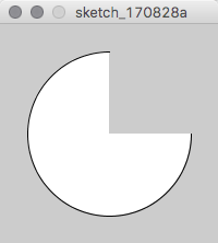
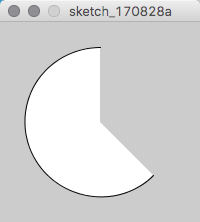
This is a weird one. It measures out in units of Pi, called radians, and the starting point on the ellipse is on the far left edge. arc(x, y, w, h, start, stop)
origin location x, origin location y,
width, height
start, stop - in radians!
Here's a version of arc() using the function radians(N) that will return a value of PI for a given value of N degrees.
Radians vs Degrees
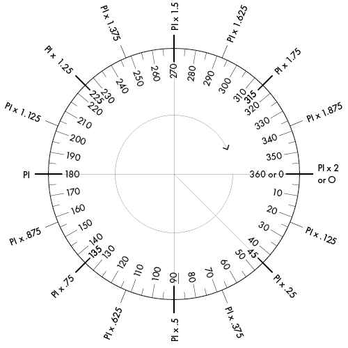
0 starts at 3:00 o'clock and runs clockwise.
PI is half way around. PI x 2 is full way around. PI x .5 is a quarter way around.
radians(Degrees) returns the correct value in terms of PI for the Degree value, so:
radians(45)
=
PI x .25
=
QUARTER_PI
radians(90)
=
PI x .5
=
HALF_PI
radians(180)
=
PI
radians(270)
=
PI x 1.5
=
PI + HALF_PI
radians(360)
=
PI x 2
=
TWO_PI
radians(30)
=
0.523599 (out of 6.23319)
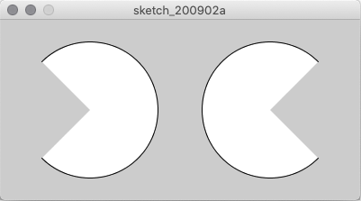
HINT: To draw an arc going counter-clockwise, use a negative starting value:
size(200,200);
// Left Pacman
arc(100,100,150,150,radians(-90),radians(180));
// Right Pacman
arc(300,100,150,150,radians(45),  radians(315));
Comments
Comments are a really big deal. Get used to commenting your code as you go along. It will save you countless hours of time when you come back to your code months later and wonder "What the hell was I trying to do here?"
Comments basically remove the commented text from being processed by the PDE, but the remain part of the Sketch file so you can keep track of your intentions
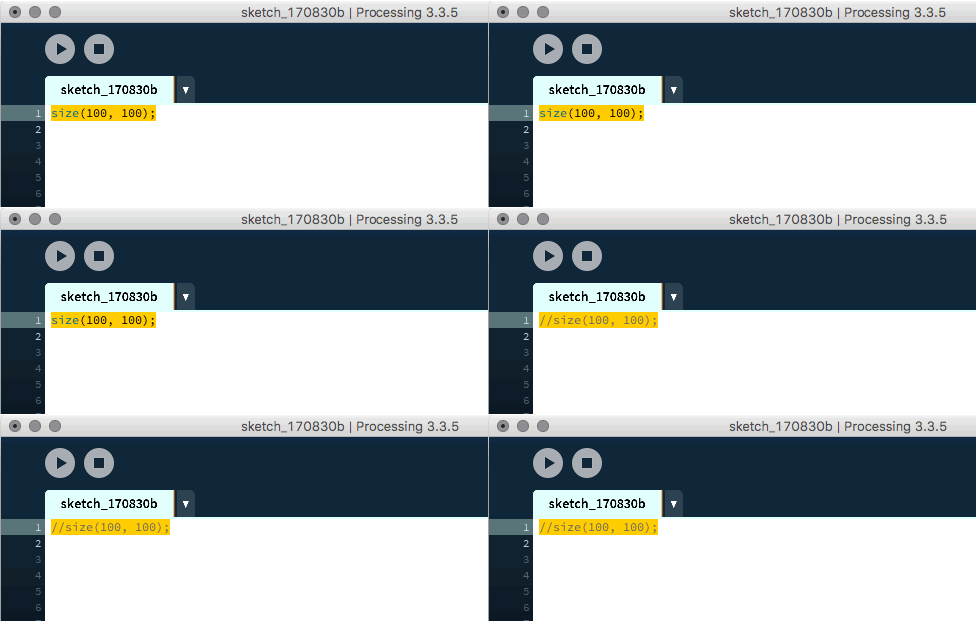
Comments are really simple, just put a double forward slash // in front of the comment. Whatever comes after the // will not be processed by the PDE until it reaches the end of the line. So this is a valid comment:
PROCESSING
Commenting with //
// This is a valid comment
size(100, 100); // This is also a valid comment
// This: size(100, 100); won't get processed because it's inside the comment
// Any comments ends at the end of the line
/* The textbook doesn't cover this yet, but using
   a forward slash followed by an asterisk starts a block of text
   that's a comment. Anything written in the sketch will be a
   comment until it's closed with an asterisk followed by
   a double forward slash */
point(50, 50);
One of the best places to use the multiline comment /* -- */ is at the top of a sketch, and use it to describe what the sketch is supposed to do, who did it, and when it was created.
PROCESSING
Commenting with /* */
/* Sketch to create a new Display Window
   that's 100 by 100 pixels.
   Created by James Khazar
   August 15, 2017
   Modified by James Khazar
   August 30, 2017 */

size(100, 100);
Another nice feature of the PDE is that you can comment and uncomment text by putting the cursor anywhere in a line and typing Control/Command-/
Very handy for de-bugging code
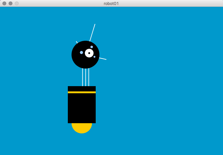
Robot 1: Draw
So here's the first robot from our book:
PROCESSING
Robot 1: Draw
size(720, 480);
smooth();
strokeWeight(2);
background(0, 153, 204);     // Blue background
ellipseMode(RADIUS);

// Neck
stroke(255);                 // Set stroke to white
line(266, 257, 266, 162);    // Left
line(276, 257, 276, 162);    // Middle
line(286, 257, 286, 162);    // Right

// Antennae
line(276, 155, 246, 112);    // Small
line(276, 155, 306, 56);     // Tall
line(276, 155, 342, 170);    // Medium

// Body
noStroke();                  // Disable stroke
fill(255, 204, 0);           // Set fill to orange
ellipse(264, 377, 33, 33);   // Antigravity orb
fill(0);                     // Set fill to black
rect(219, 257, 90, 120);     // Main body
fill(255, 204, 0);           // Set fill to yellow
rect(219, 274, 90, 6);       // Gray stripe

// Head
fill(0);                     // Set fill to black
ellipse(276, 155, 45, 45);   // Head
fill(255);                   // Set fill to white
ellipse(288, 150, 14, 14);   // Large eye
fill(0);                     // Set fill to black
ellipse(288, 150, 3, 3);     // Pupil
fill(153, 204, 255);         // Set fill to light blue
ellipse(263, 148, 5, 5);     // Small eye 1
ellipse(296, 130, 4, 4);     // Small eye 2
ellipse(305, 162, 3, 3);     // Small eye 3